Background on Project
Last year, on this project, a similar implementation of the model by Google was done and the results regarding the same were obtained. A detailed summary regarding the background of the project is available on -https://dssr2.github.io/gaze-track/ . Below is the explanation for some useful terms frequently used in this report.
Important Terms
- .tfrec file
The TFRecord format is a simple format for storing a sequence of binary records.
- Gazetrack dataset
The main dataset whose split and directory structure are explained below.
- Google Model
The .tflite model provided by Google for experiment purposes.
- SVR
Multi-Regression Support Vector Machine
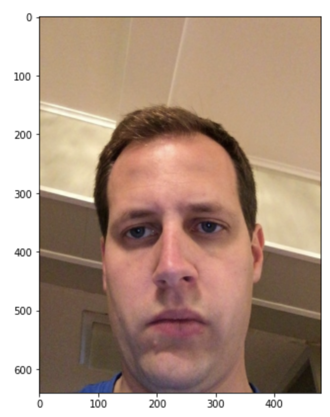
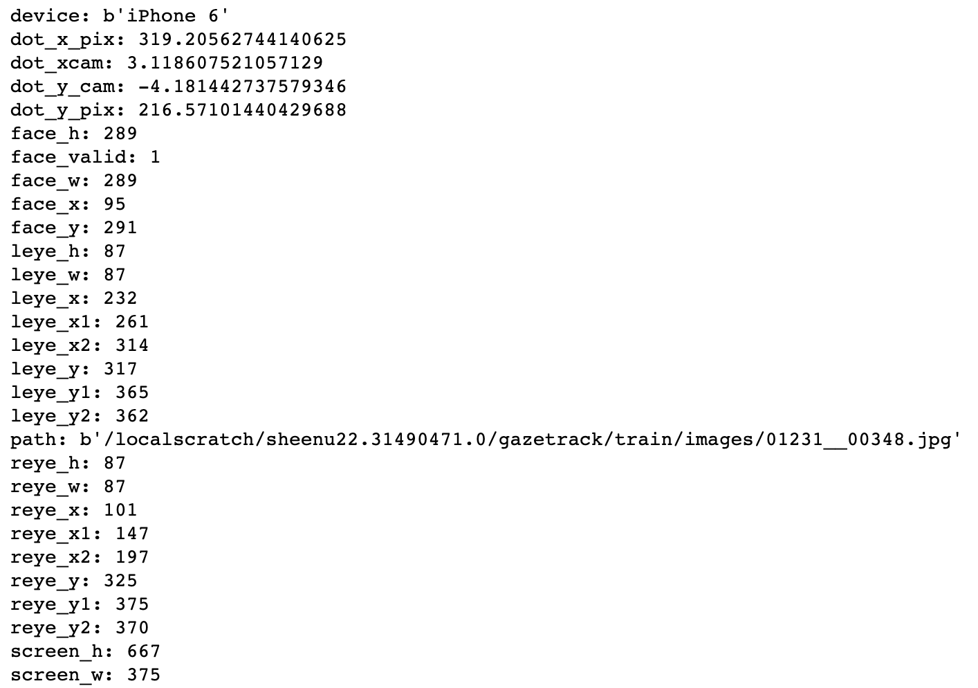
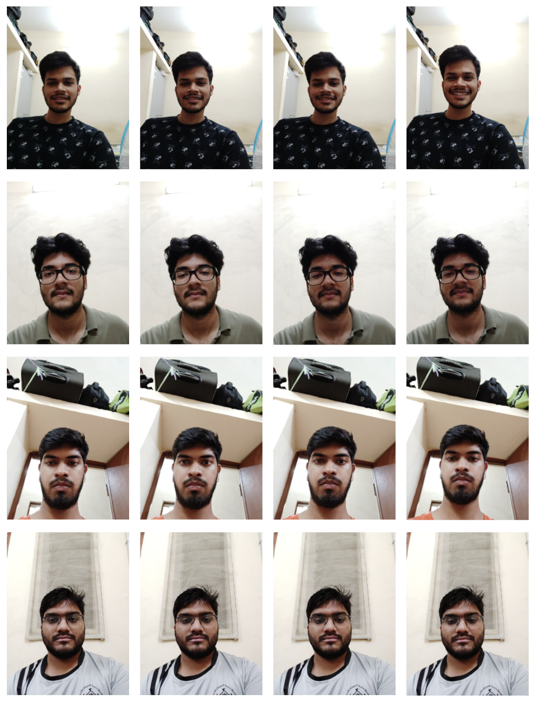
- Individual Datapoint (gazetrack)
The visualization of a tfrec data point is given below.
- MED - Mean Eucledian Distance
Main Idea
To perform various experiments on the Google’s Tflite model to reimplement the results in Accelerating eye movement research via accurate and affordable smartphone eye tracking and analyze the trend of MED on the .tflite model after various versions of SVR. Code for the project is present here
DATASETS
Main Datsets and Splits
This project is based on different versions of the massive Gazecapture Dataset from MIT.
Major portion of my work has been on a smaller version of the same dataset -
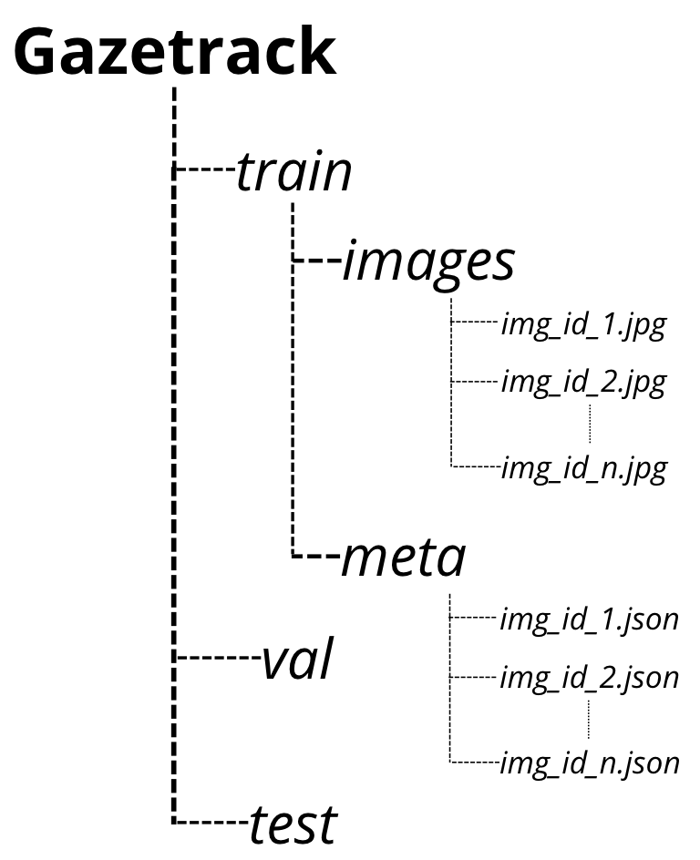
gazetrack.tar.gz. The directory structure of the dataset is explained below.
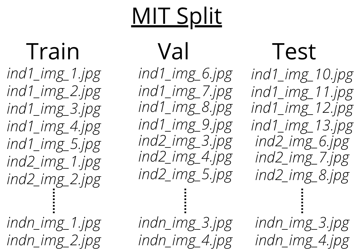
There are two splits that are available for the same dataset - MIT Split and Google
Split. MIT split contains frames of unique individuals in each train, val, and test set.
This means that the frames corresponding to an individual are present in either train or
val or test.
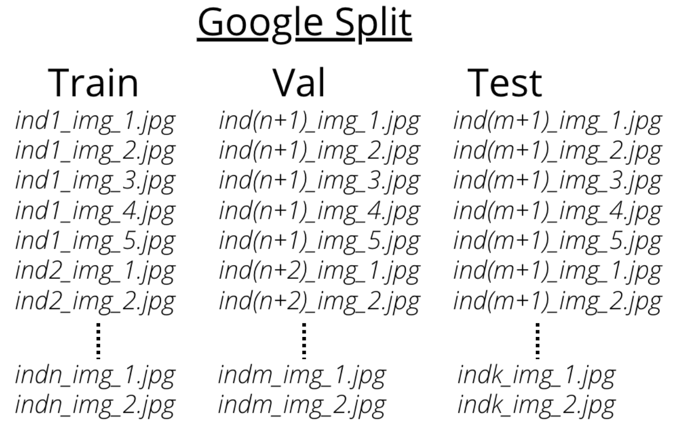
Google Split contains frames of individuals across the train, val and test set. This
means that the frames corresponding to an individual are present in train and test and
val set.
Main Tfrec dataset
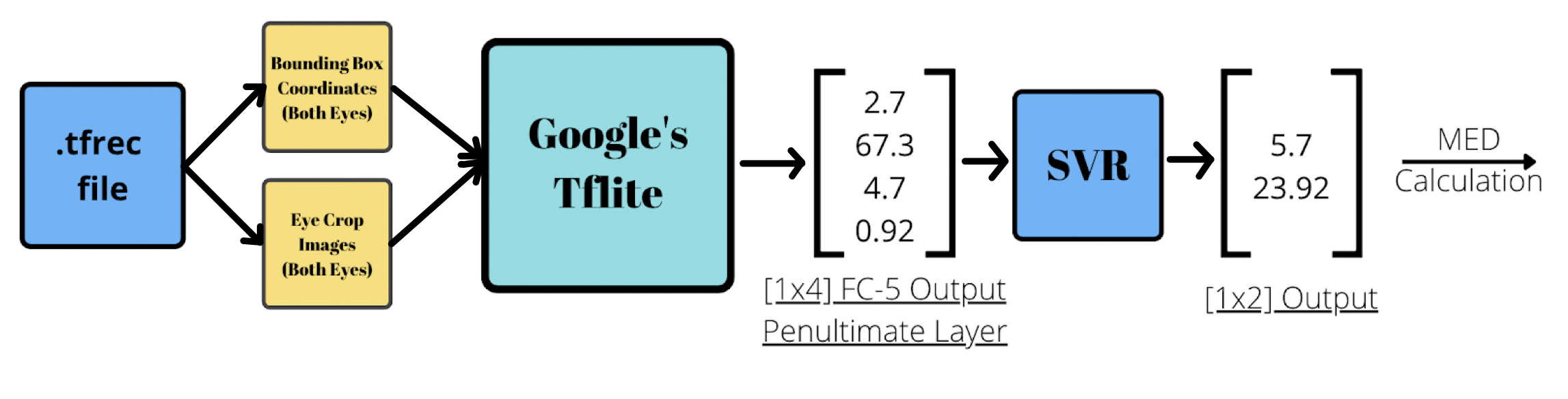
In order to completely implement the Google Model’s Input Pipeline for inference, the dataset should be saved as a .tfrec file and images be read through tf.example protocol buffer from the .tfrec and then the further processing on image can be done. So then I created a .tfrec based dataset from the already existing gazetrack.tar.gz dataset on the server.
The link for tfrec dataset creation is
https://github.com/prakanshuls22/GSoC_2022_INCF/blob/main/GSoC_22/Tfrec_creation_main.py
Individual and Combined tfrec datasets
Google had performed per user per block SVR personalisation. Now to perform this per user
SVR training and testing, the outputs of the .tflite model had to be segregated by users
which meant that the .tfrec files had to be arranged according to users.
Thus I created .tfrecs suited to the same. A combined .tfrec file containing ten
individuals with all the frames from test train and val of gazetrack.tar.gz. Also these
ten individuals were chosen on the basis of - number of frames per user, i.e, these 10
individuals have the highest number of frames among all the users in the gazetrack
dataset combined (test train and val).
The results of the .tflite model on this .tfrec were then fed into SVR for per user
personalisation.
The link to this SVR per user personalisation is here.
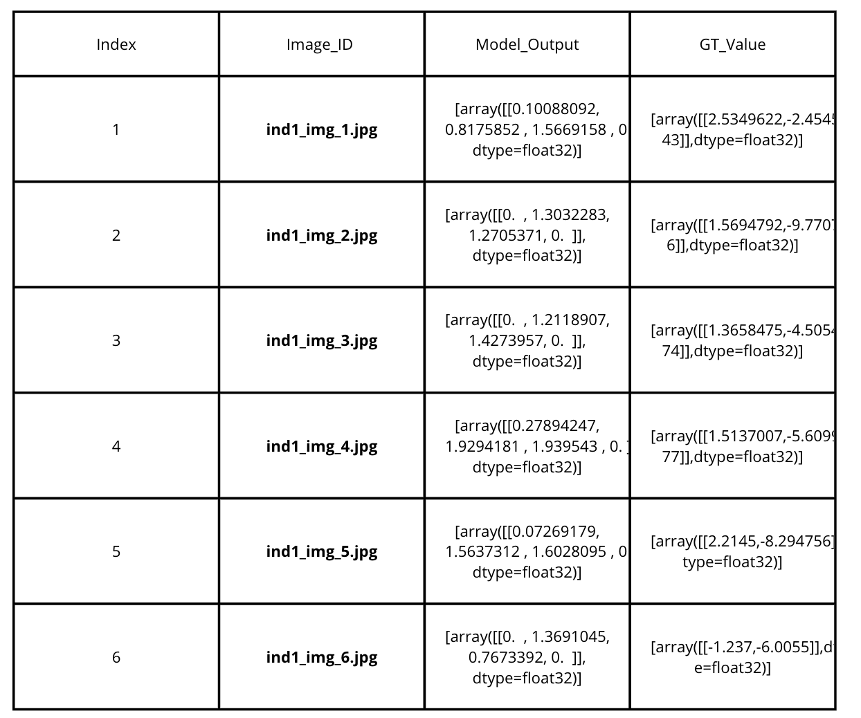
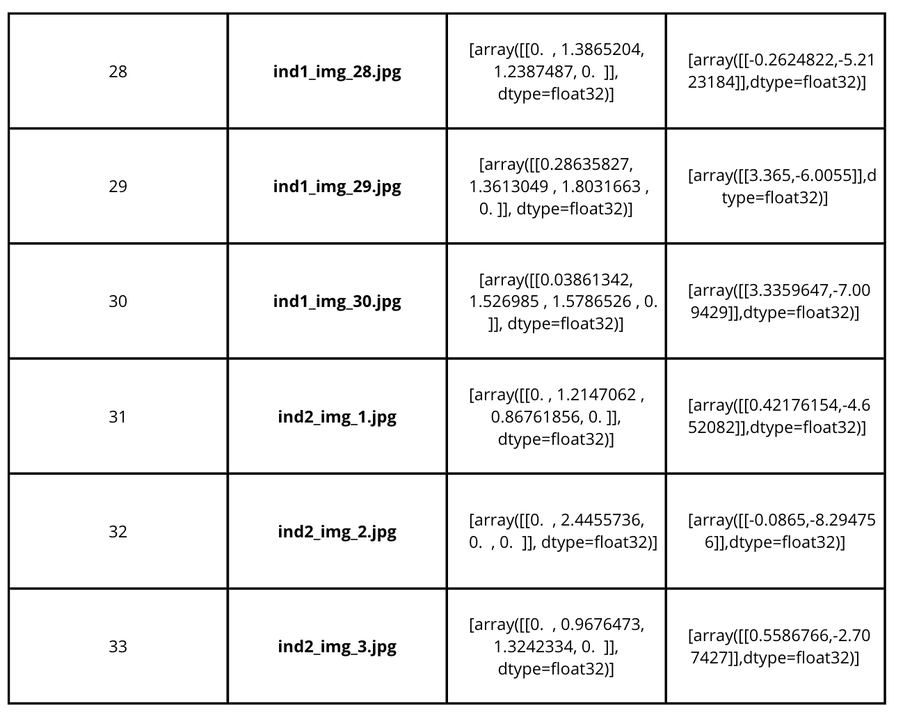
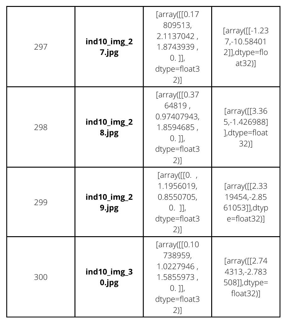
Unique 30 dataset (csv)
To carry out an experiment performed last year on the same project, we ran the SVR on
Google model’s output on 30 unique gazetrack points per individual. For the same unique
points for every individual were extracted from all the CSV outputs for google
model.
The structure of the unique points CSV is elaborated in the image below for better
understanding.
MODEL/VERSIONS
Google .tflite version
This version was provided by Google itself. We had experimented extensively with this version and the results are visualized below in the report.
Keypoints and Eye bounding box
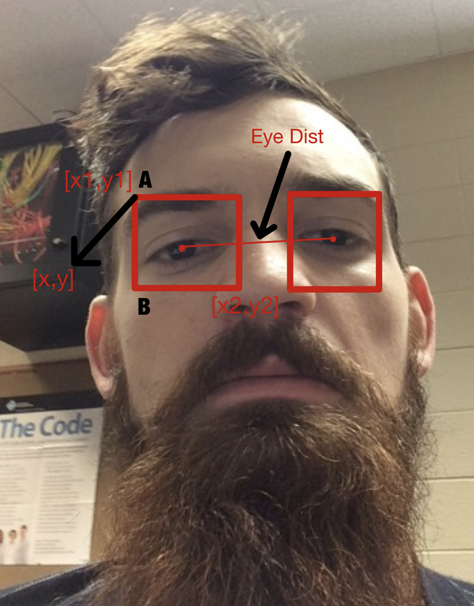
The image on the left defines the different points that are used in the table below. A refers to the top left point of the bounding box where as B refers to the bottom left point of the bounding box. The Eye Dist in the image on the left is represented by 'e' in the table below. w and h in the below table refer to the width and the height of the bounding boxes of the eyes. 'S' in the 'BOUNDING BOX POINTS ALIGNMENT' refers to the swapped keypoints for that input version. By swapping I mean, that we provide left keypoints for the right eye and vice versa. This is done to test both the possible right and left combination of eyes - as viewed by an user through an image and the original position of the eye.
Experimental Versions
| Version/Modification | Bounding Box Points Alignment | Bounding Box Format | Eye Crop Size | Bounding Box as input | Bounding Box Normalization | Input Sequence to Model | Dist Function |
|---|---|---|---|---|---|---|---|
| v0 | Default | [x,y,w,h] | Original | Bottom Left | By Screen Size | (rb,lb,re,le) | NA |
| v1 | Default | [x,y,w,h] | Original | Bottom Left | By Image Size | (rb,lb,re,le) | NA |
| v2 | Default | [x,y,w,h] | Original | Top Left | By Image Size | (rb,lb,re,le) | NA |
| v3 | Default | [x,y,w,h] | e/2, e/2 | Bottom Left | By Image Size | (rb,lb,re,le) | np.linalg.norm |
| v3b | S | [x,y,w,h] | e/2, e/2 | Top Left | By Image Size | (rb,lb,re,le) | np.linalg.norm |
| v3testing | Default | [x,y,w,h] | e/2, e/2 | Bottom Left | By Image Size | (rb,lb,re,le) | math.dist |
| v4 | Default | [x,y,w,h] | e/2, e/2 | Top Left | By Image Size | (rb,lb,re,le) | np.linalg.norm |
| v4b | S | [x,y,w,h] | e/2, e/2 | Top Left | By Image Size | (rb,lb,re,le) | np.linalg.norm |
| v4testing | Default | [x,y,w,h] | e/2, e/2 | Top Left | By Image Size | (rb,lb,re,le) | np.linalg.norm |
| v5 | Default | [x1,y1,x2,y2] | e/2, e/2 | Top Left | By Image Size | (rb,lb,re,le) | np.linalg.norm |
| v5b | S | [x1,y1,x2,y2] | e/2, e/2 | Top Left | By Image Size | (rb,lb,re,le) | np.linalg.norm |
| vfinal | Default | [x,y,w,h] | e/2.5, e/3 | Top Left | By Image Size | (lb,rb,le,re) | abs |
| vfinal_unif | Default | [x,y,w,h] | e/2.5, e/3 | Top Left | By Image Size | (lb,rb,le,re) | abs |
| vfinal_flipkey | S | [x,y,w,h] | e/2.5, e/3 | Top Left | By Image Size | (lb,rb,le,re) | abs |
| vfinallrnoflip_flipkey | S | [x,y,w,h] | e/2.5, e/3 | Top Left | By Image Size | (rb,lb,re,le) | abs |
| vfinallrnoflip | Default | [x,y,w,h] | e/2.5, e/3 | Top Left | By Image Size | (rb,lb,re,le) | abs |
App Data Collection
A small instance of data collection was also done during the project. Data was collected through an app (android .apk). This data would be later used in the project for fine tuning our own trained model on the same lines as Google, and then the comprehensive comparison can be carried out for an end to end model for Gazetracking.
SVR
SVR (sklearn.svm.SVR) was used by google to further map its penultimate layer output in another tensor space, and then further used this mapped tensor to calculate the Mean Euclidean Distance. In this implementation also, SVR is used for the same.
Per-User personalisation - In this SVR execution, the outputs for a single individual are consolidated and then split into train and test set, and then SVR is fitted on the train set (against gaze ground truth value), and tested for the MED on the test set.
SVR was performed on different dataset splits and folds mentioned below.
- Folds - 3 fold and 5 fold cross validation strategy
- Split- Google Split (Fig reference)
- Split Sequence
First - First split the corresponding dataset in 70/30 train/test ratio, and then fitting the SVR on the train and then testing on test.
Later - fitting on the corresponding dataset (in the two folds mentioned above) and extracting the best hyperparameters, and then tuning on those parameters on a 70% train division and then testing it on a 30% test division.
- Epsilon Range
A lower and higher epsilon range has been swept through as an experiment. Higher range corresponds to more values between the interval of sweep for epsilon. For example - 0.1,0.2......1,2....10,20,30....100,200,300....1000. Whereas a lower range corresponds to less values between the interval of sweep for epsilon. For example - 0.1,1,10,100,1000.
Results and Visualizations
MED for 10 different users and the average for all those individuals was plotted across all the different versions for input to the google model and this is how the plots came out to be -
The legends for all the below plots is -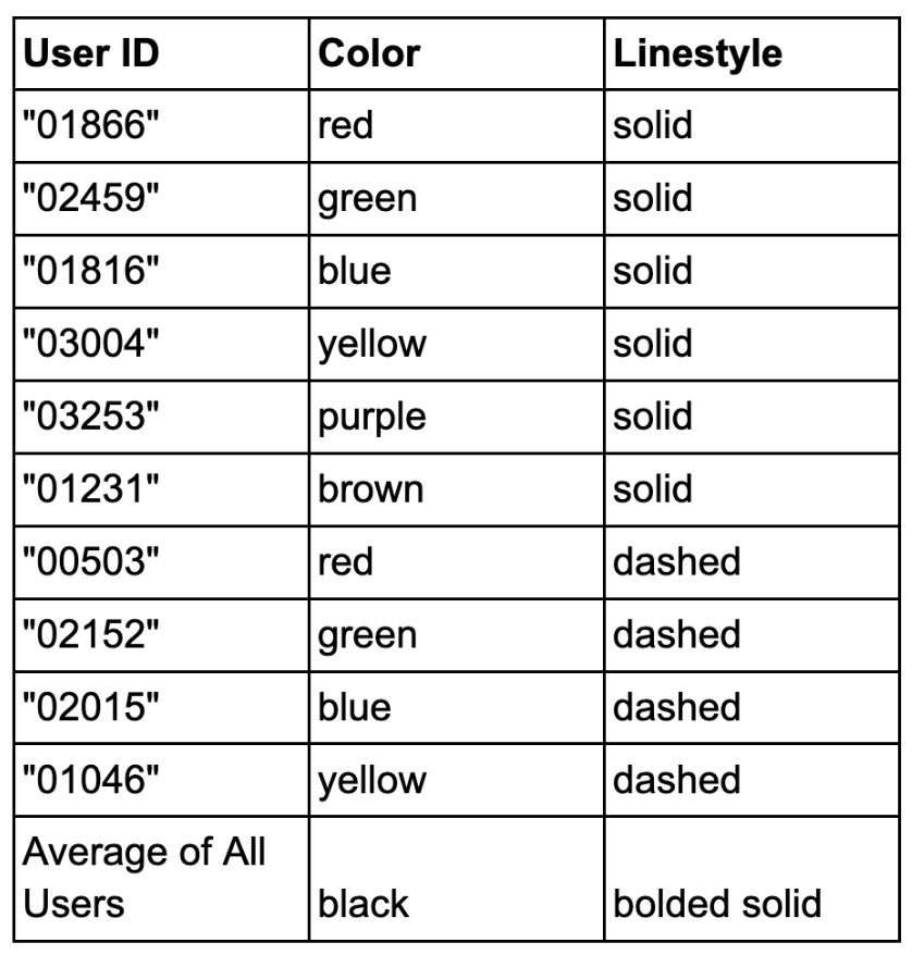
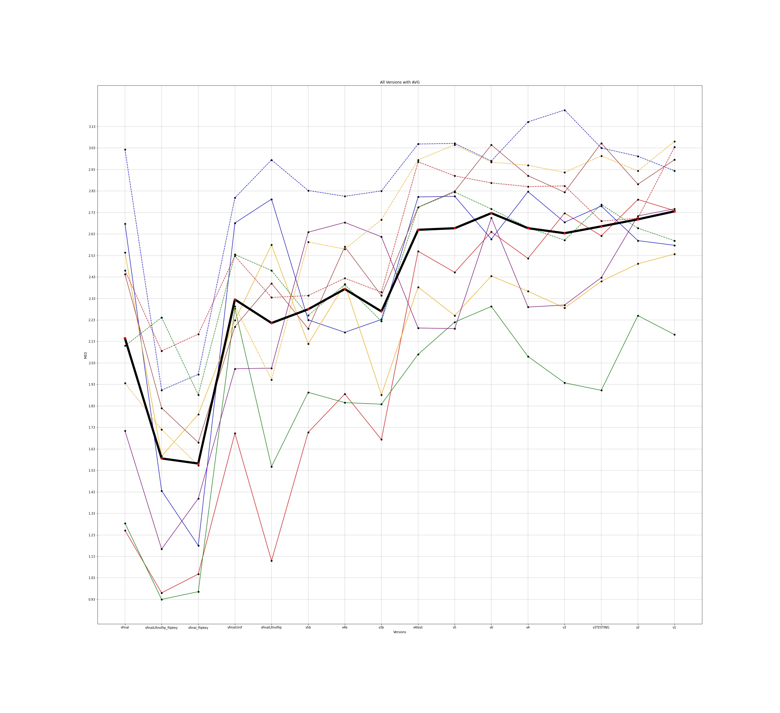
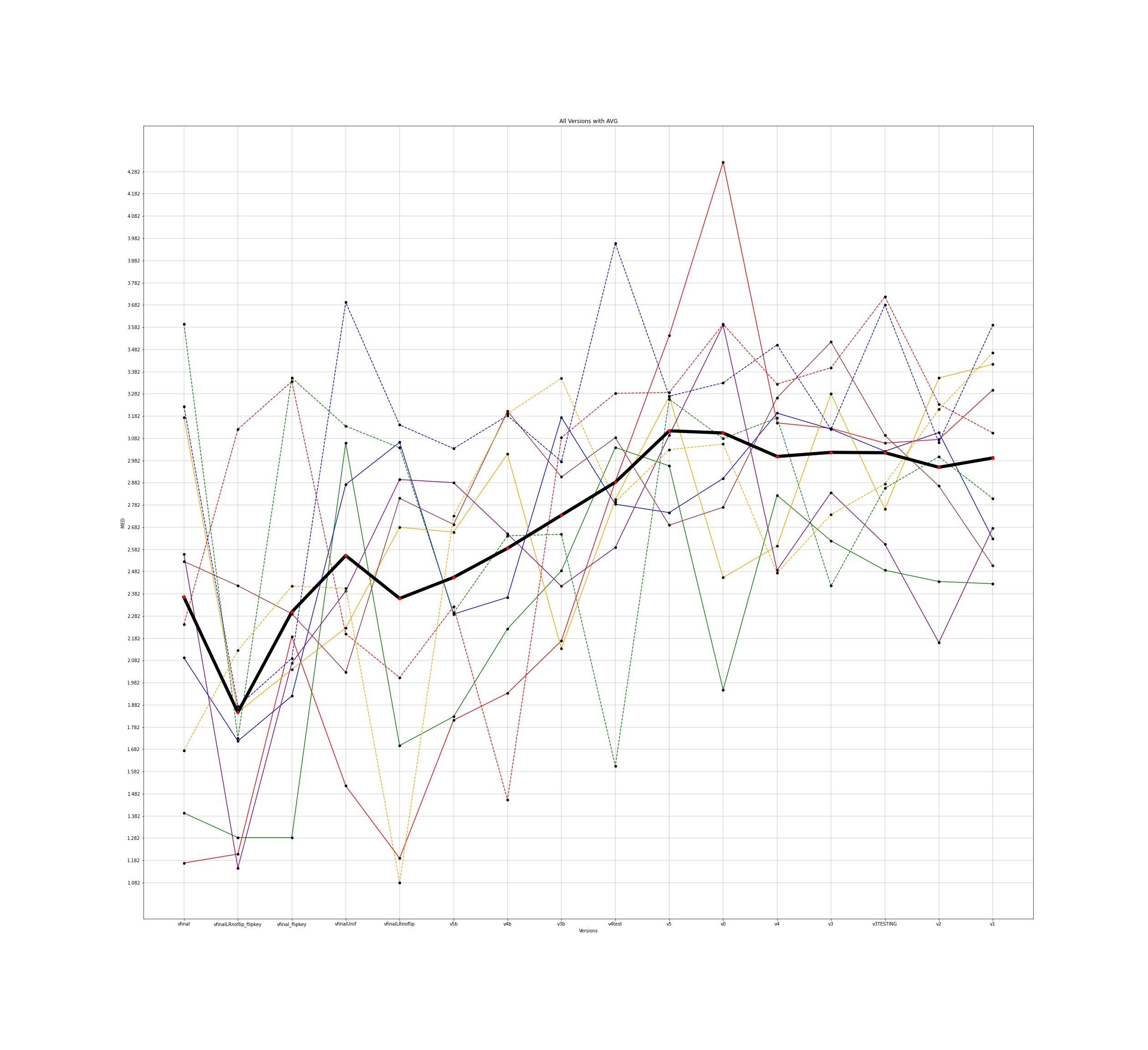
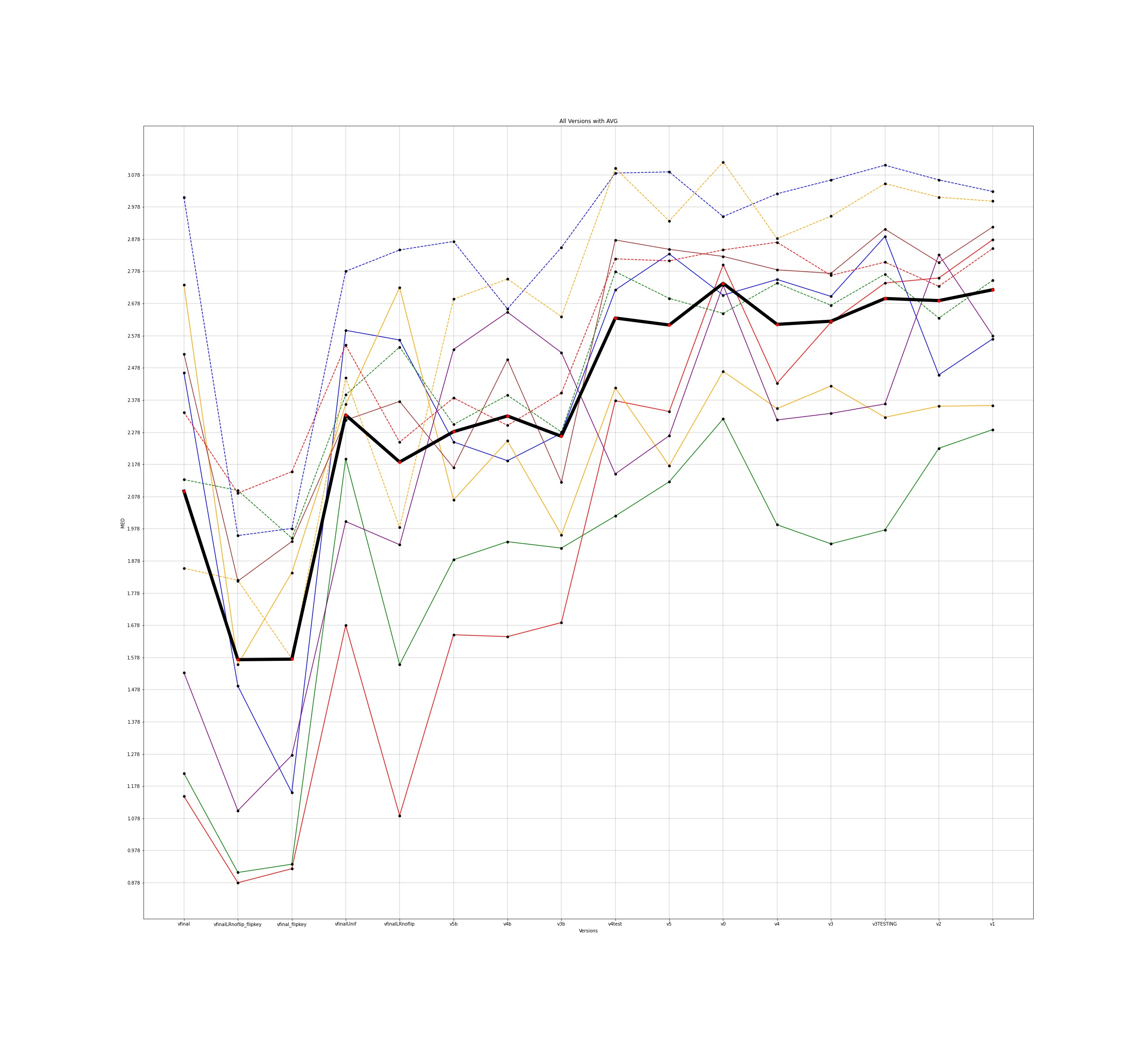
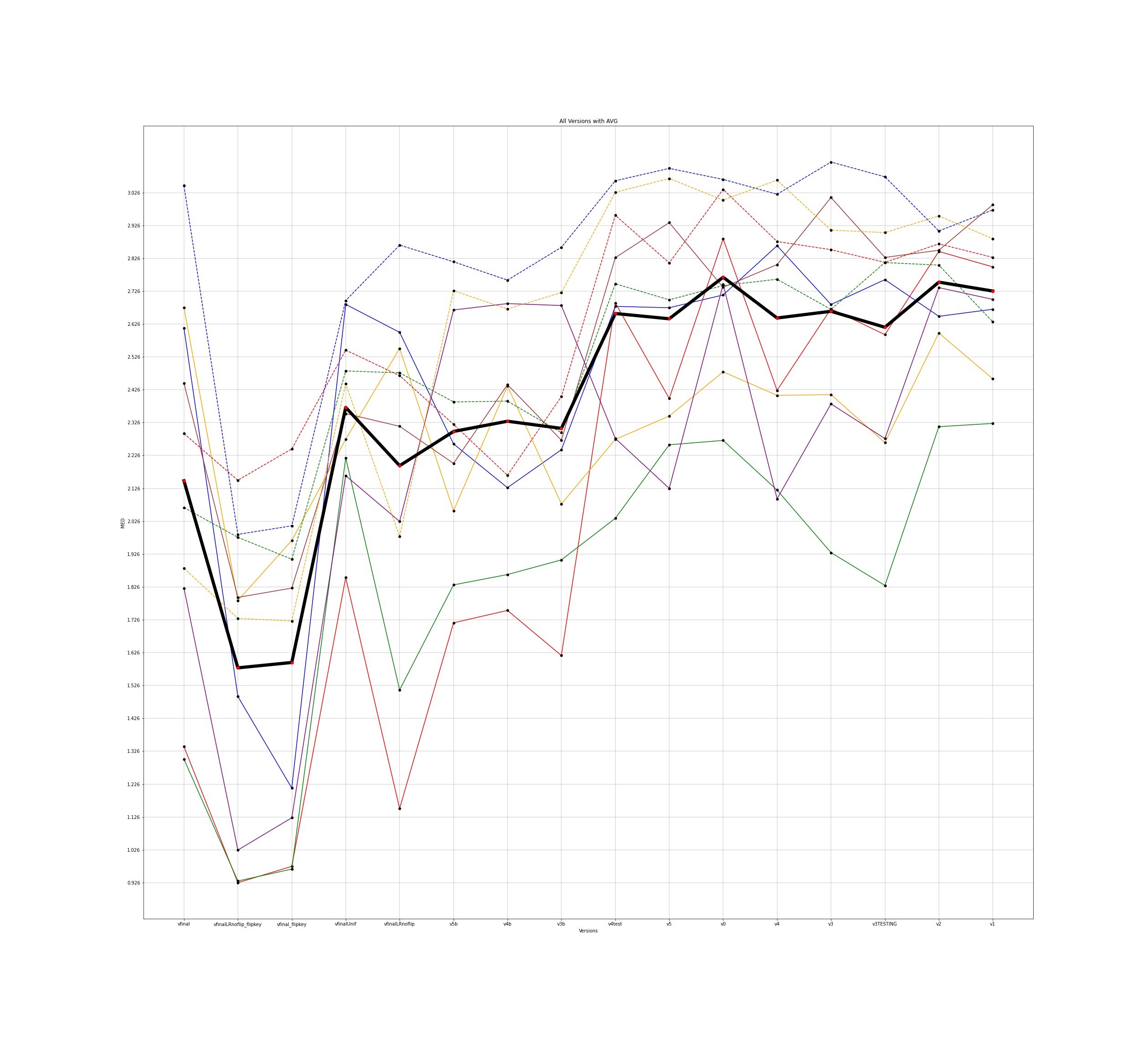
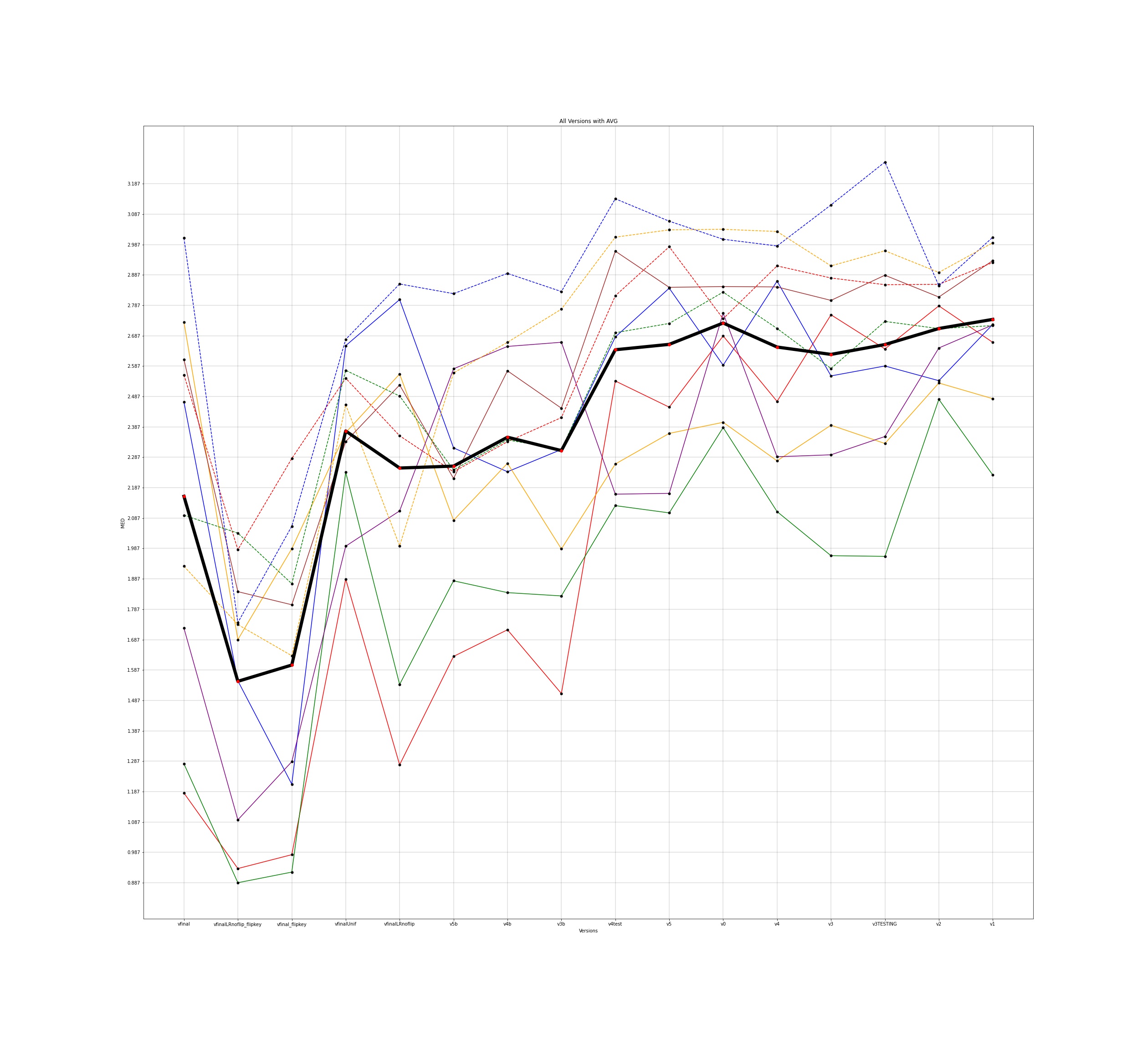
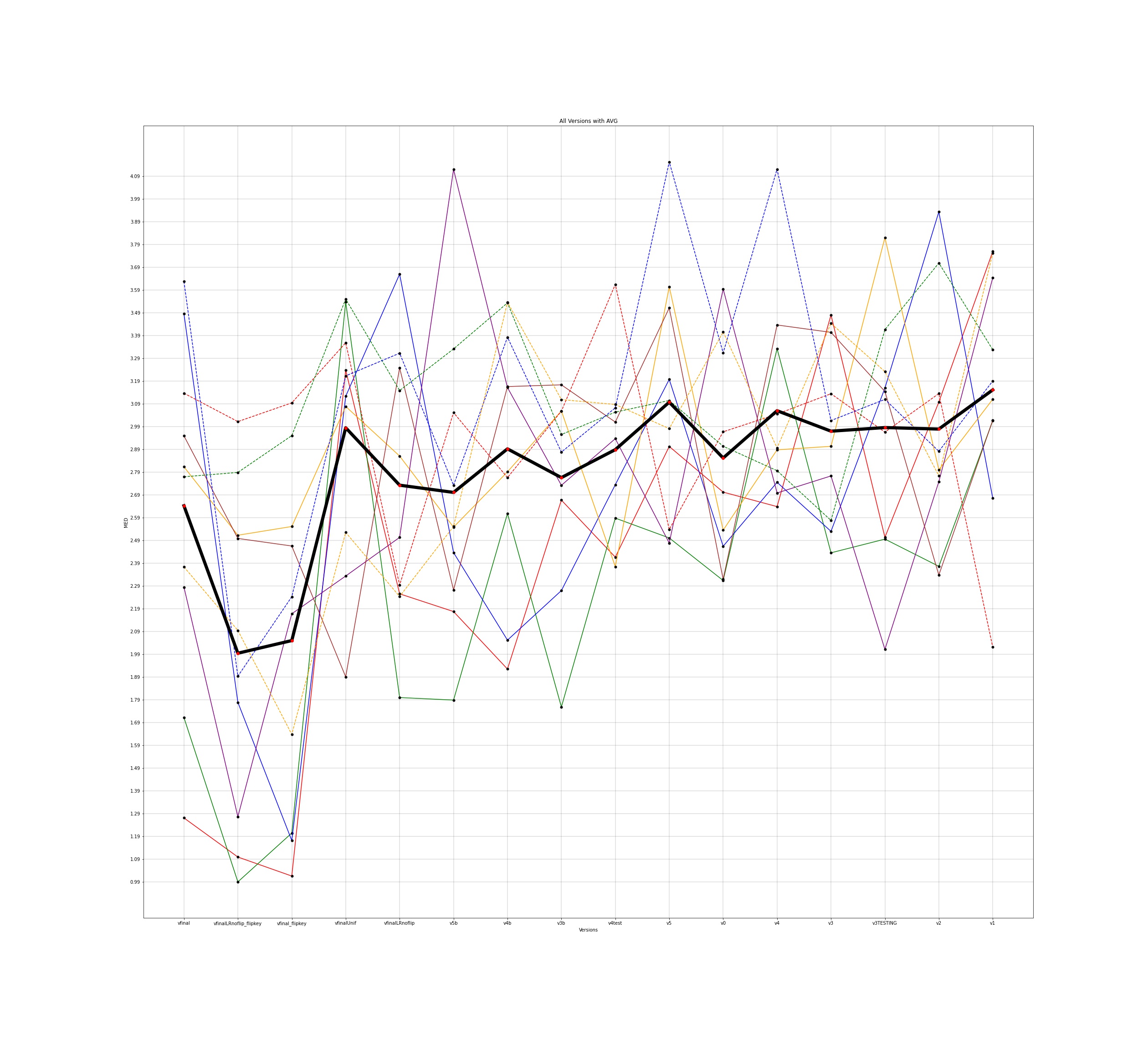
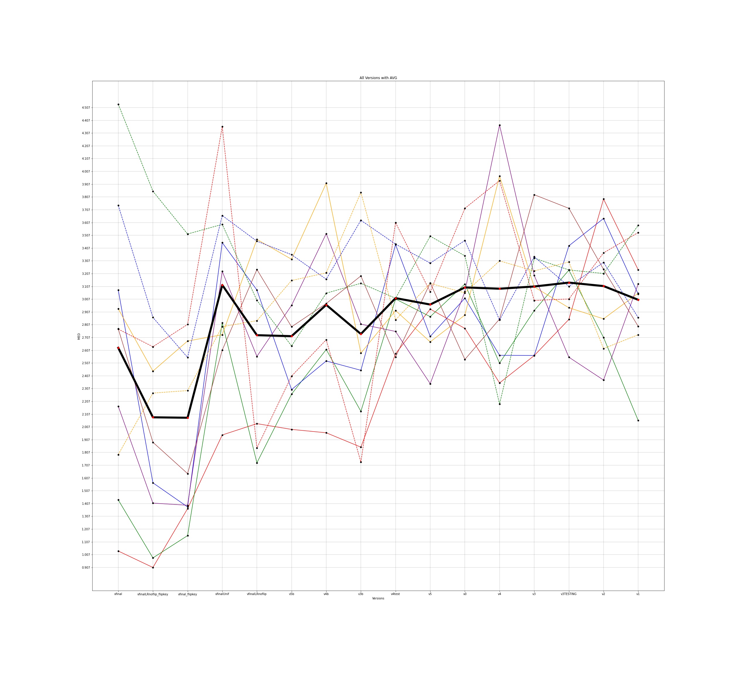
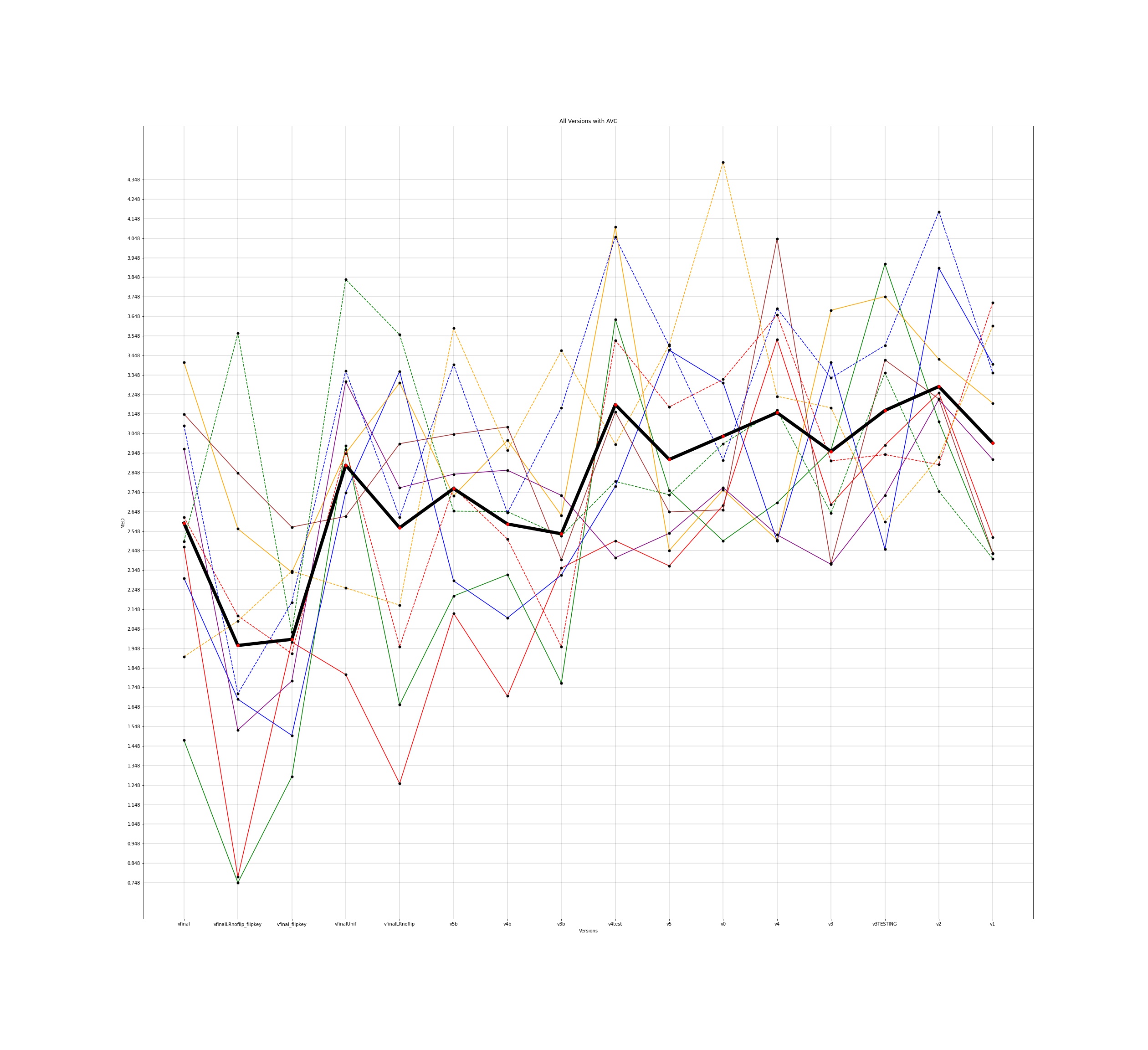
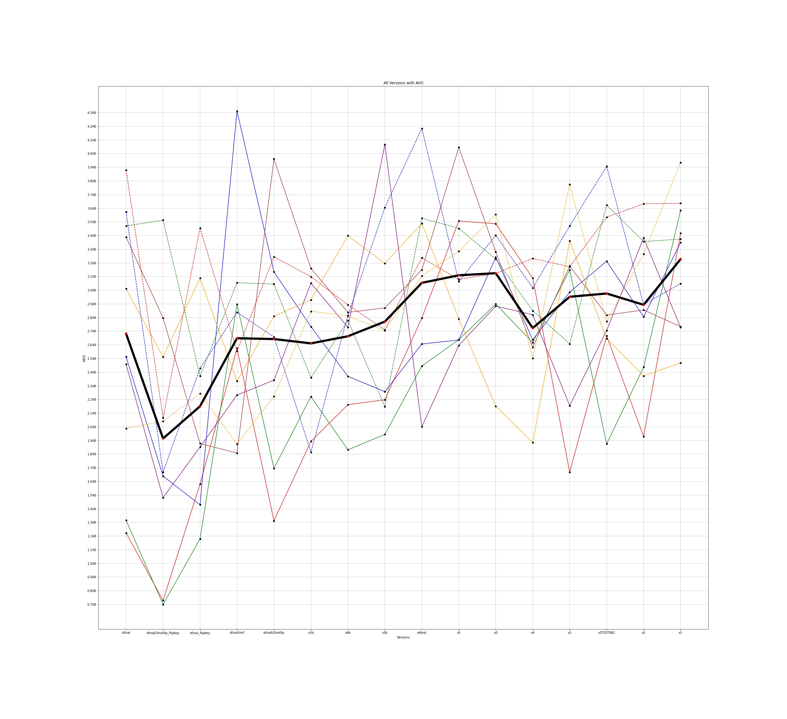
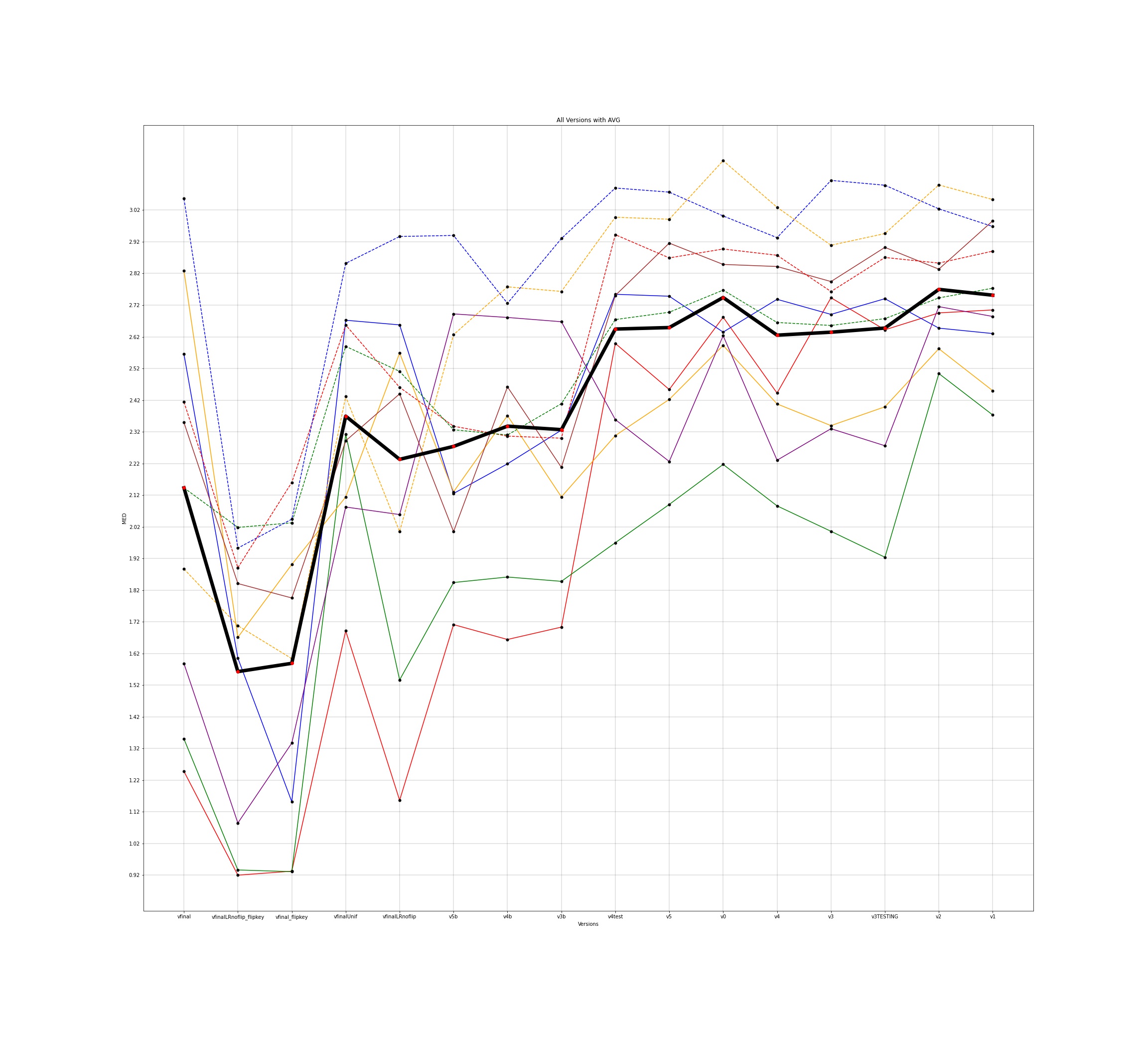
The notebooks for the visualisations are present here
Challenges and Learnings
Challenges
No previous significant experience in Tensorflow.
Learnings
-
Working with larger datasets
-
Working with Tensorflow to all the way to the basic implementations
-
Writing and modifying code according to the situation/requirement of the team/organization
-
Working of SVR (fitting and sweeping)
Conclusion and Future Direction
The project is completed as major experimentations on the google model and the input version with the lowest error have been determined. Now lies ahead, further testing the model’s accuracy on our set of calibration data that we have collected throughout this project. Incorporation of face-filter and face-tilt features can be tested with the current version of google base model to try and further decrease the MED for gaze estimation.